Machine Learning using RandomForestRegression
Introduction
In this project I use Airbnb data to analyze their price distribution and to create a machine learning model that can be used to predict the price of a given listing. Airbnb data for major cities and towns around the world is publicly available at Inside Airbnb project. For this analysis, I work with the data for Berlin, Germany.
1. Overview
First, we download the data from this link. The file listings.csv.gz has all the data that we need but the other files are also useful for further analysis and visualization.
Once we have the data we need, we can start our exploratory analysis.
Let’s import the modules and load the data as shown here.
In the code above, we imported:
- Pandas and Numpy for data processing
- Matplotlib & Seaborn for visualizing our data
- Train_test_split for spliting our data into sets for training and testing our model
- RandomForestRegressor for creating a regression model. This is a supervised machine learning task and RandomForest is a good candidate for it. Based on the performance of our model in predicting apartment prices, we might also try other algorithms for comparison
- Mean_squared_error and mean_absolute_error for measuring the performance of our model
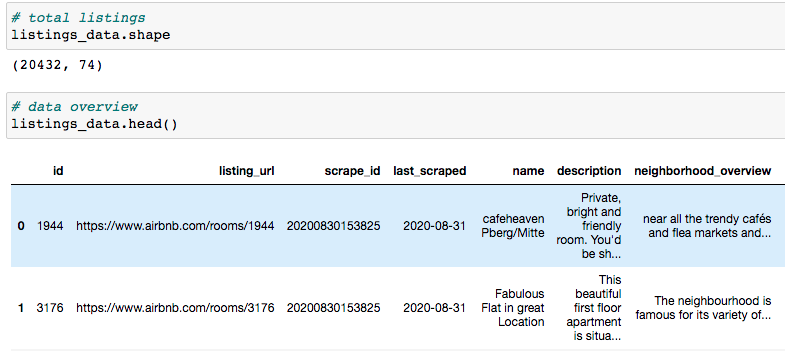
Let’s take a quick look at the shape and overview of our data.
As shown below, we have 20432 listings and 74 columns (features).
2. Data Processing
Let’s remove the currency notation from the prices using this function
Once prices are cleaned up we can look at their distribution
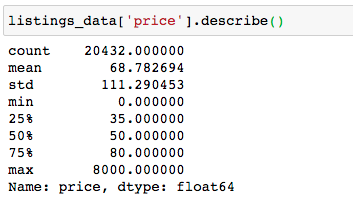
We can make the following observations:
- The average cost cost of renting an apartment is $68 and the median price is $50
- Prices range from $0 to $8000
- 75% of the listings cost $80 or less per night
- Only 4.98% of the listings cost more than the 95th percentile price ($155)
- Only 0.4% of the listings cost $500 or more
3. Exploratory Data Analysis
Let’s plot the price distribution
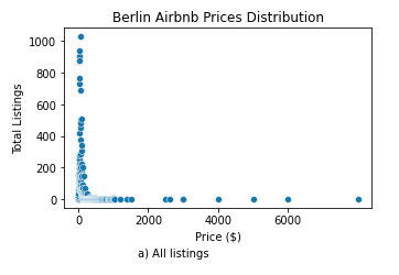 |
| 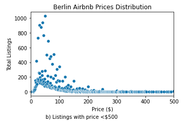
- In the second graph we zoom in on apartments that cost less than $500
3.1 Price Comparison
Let’s take a look at how some of the features such as distance from the city center, number of bedrooms, room type and neighbourhood affect prices
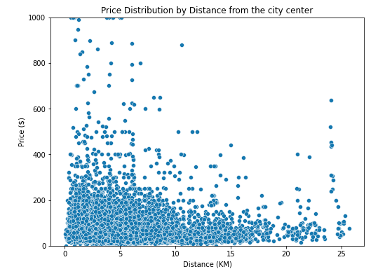
a) Distance from city center
Let’s calculate the distance from the city center. For Berlin we will use Alexendarplatz square in Central Mitte District as the center. Using the following function, we calculate the Great-circle Distance in kilometers for all the apartment listings using the harvesine formula.
- Based on the following distribution, we can see that prices generally decrease as you move away from the city center
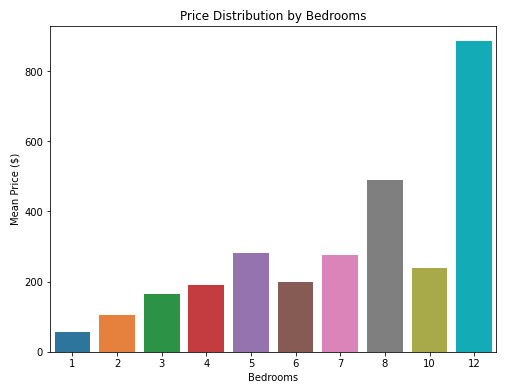
b) Number of bedrooms
- One bedrooms apartments are the cheapest on average
- The average prices linearly increases for apartments with 1-5 bedrooms but fluctuates for apartments with 6 or more bedrooms. This could be a sign of anormalies or outliers pricing for apartments with the highest number of bedrooms
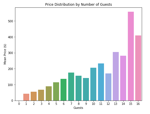
c) Maximum number of guests
- As expected, price increases with the number of guests
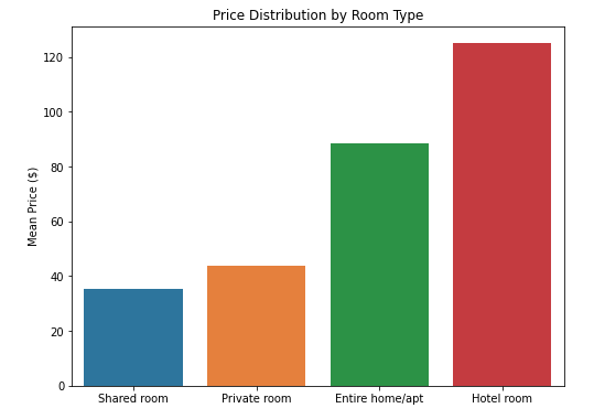
d) Room Type
- It’s cheaper if you shared the apartment with the host
- Hotel rooms are the most expensive on average
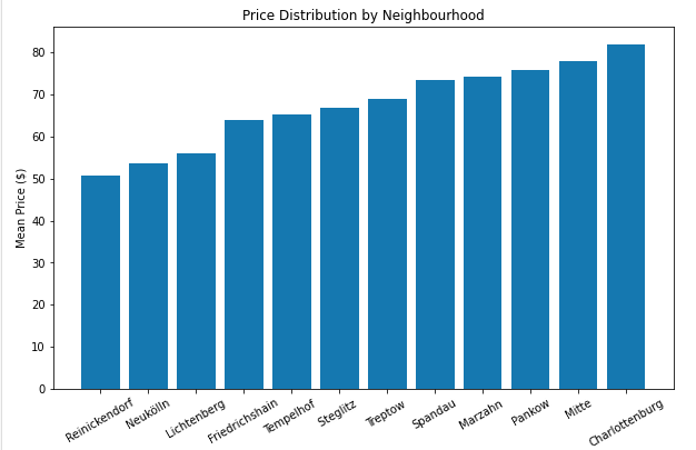
e) Neighbourhood
- Apartments in Charlottenburg ($81) are the most expensive followed by Mitte boroughs ($71)
- Reinickendorf has the the cheapest apartments
4. Feature Selection
We have looked at how some of the features affect pices. In this section, we are going to determine which other features in our dataset greatly affect the price of renting an Airbnb apartment.
i) Missing Values
First let’s check which columns have the highest number of values missing
This table shows the top ten columns with the highest number of missing values
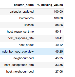
- We have another column named bathrooms_text so we shouldn’t worry about bathrooms
- We have 9 columns with more than 30% values missing. We’ll drop these columns
- We also have 14 columns with between 5% and 30% values missing
- For integer columns with missing values, we impute the missing values using the median strategy. In this case, we fill the missing values in a column with the calculated median for that column
- For categorical columns, we will add an ‘uknown’ class to the data
ii) Feature Importance
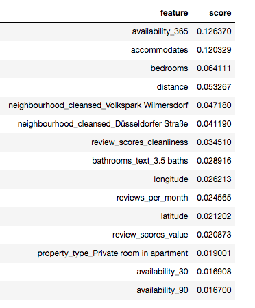
Now we need to determine the best features to use in our model. We will use a RandomForestRegressor to fit our feaures and the target variable then we calculate the feature importances. The code below shows how to find important features
Here are the top 15 features and their scores
5. Model Selection
a) Fit the model
Using the top features, we can train our final model. We either select top n features or we select features with scores above a certain threshold then we train several models to compare performances
As shown below, we selected 50 features to the model
b) Make predictions
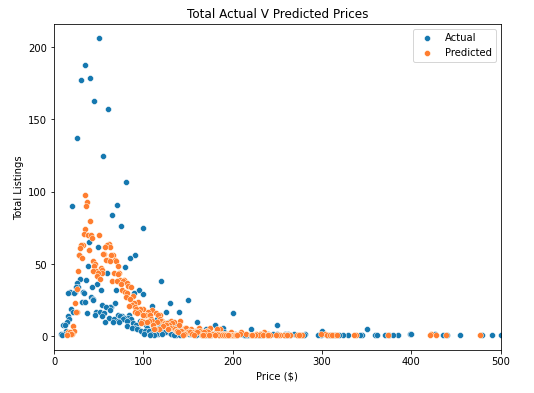
Once our model is trained, we use it to make predictions
- Then we score the performance of our model using both the mean squared errors and the mean absolute error
- The model returned an R^2 of 5.3% which means it’s not doing a great job at explaining the variance in our data
- We also have a RMSE (Root Mean Squared Error) of 147.5 which indicates that in a given prediction, our model is missing the prediction by $147
- Similarly our MAE (Mean Absolute Error) is 25.5
- This model needs further tuning in order to improve our prediction results.
Looking at the results however, we can see that our predicted prices closely match the actual prices.
Conclusion
In this analysis, we looked at how a RandomForestRegession model performs given a set of features. We definitely need to further tweak the model parameters in order to improve performance. We can also try other regression models like XGBoost for comparison.